Masses, Star Formation Efficiencies, and Dynamical Evolution of 18,000 H II Regions

Published in The Astrophysical Journal Letters, Volume 993, Issue 1, id.L20, 14 pp., 2025

Abstract

We present measurements of the masses associated with ∼18,000 H II regions across 19 nearby star-forming galaxies by combining data from JWST, Hubble Space Telescope, MUSE, Atacama Large Millimeter/submillimeter Array, Very Large Array, and MeerKAT from the multiwavelength PHANGS survey. We report 10 pc-scale measurements of the mass of young stars, ionized gas, and older disk stars coincident with each H II region, as well as the initial and current mass of molecular gas, atomic gas, and swept-up shell material, estimated from lower-resolution data. We find that the mass of older stars dominates over young stars at ≳10 pc scales, and ionized gas exceeds the stellar mass in most optically bright H II regions. Combining our mass measurements for a statistically large sample of H II regions, we derive 10 pc-scale star formation efficiencies of ≍6%─17% for individual H II regions. Comparing each region's self-gravity with the ambient interstellar medium (ISM) pressure and total pressure from presupernova stellar feedback, we show that most optically bright H II regions are overpressured relative to their own self-gravity and the ambient ISM pressure and that they are hence likely expanding into their surroundings. Larger H II regions in galaxy centers approach dynamical equilibrium. The self-gravity of regions is expected to dominate over presupernova stellar feedback pressure at ≳130 and 60 pc scales in galaxy disks and centers, respectively, but is always subdominant to the ambient ISM pressure on H II region scales. Our measurements have direct implications for the dynamical evolution of star-forming regions and the efficiency of stellar feedback in ionizing and clearing cold gas.

Figures
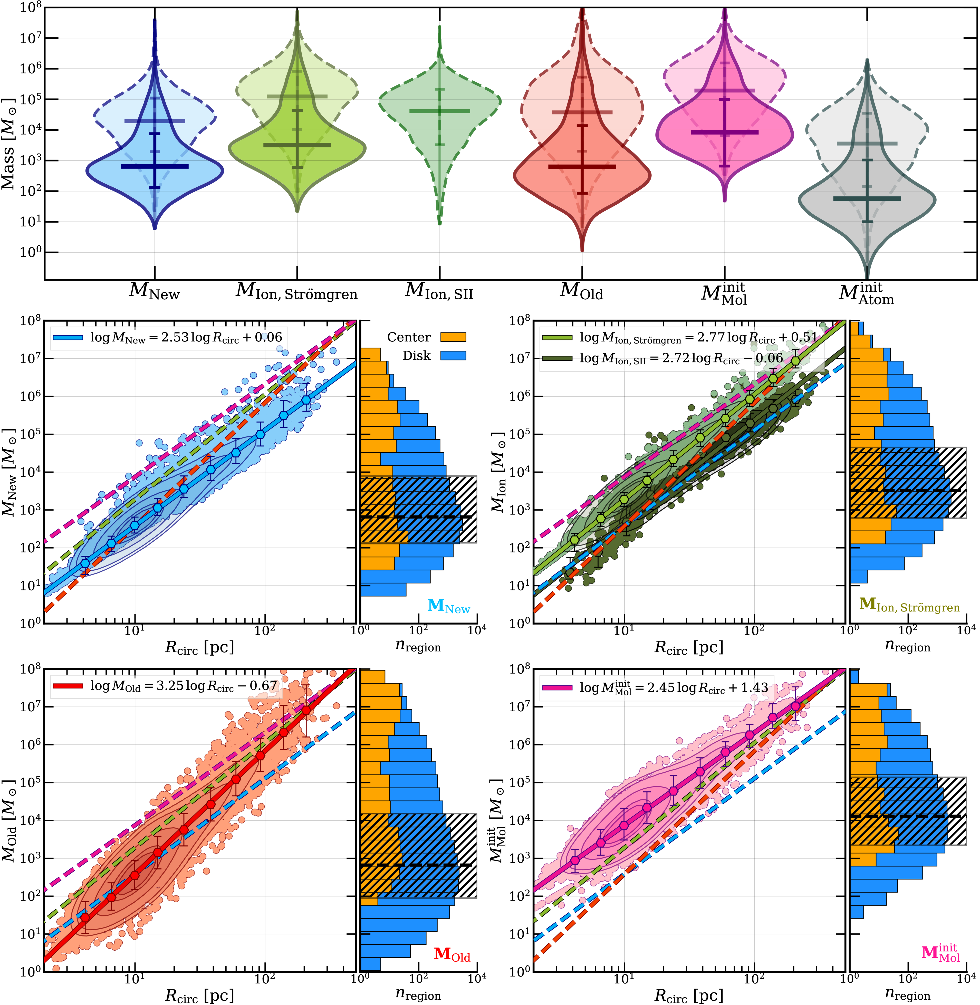
Figure 1. The distribution of masses associated with our sample of ∼18,000 H II regions (solid violins) and the subsample of ∼4000 regions where we can calculate [S II] densities (dashed violins), including contributions from young clusters (MNew, in blue; see Section 2.1.1), ionized gas mass (MIon, Strömgren in light green and [S II]-emitting clump in dark green; see Section 2.1.2), old stellar mass (MOld, in red; see Section 2.1.3), initial molecular gas mass (﹩{M}_{{\rm{Mol}}}^{{\rm{init}}}﹩, in pink; Section 2.2.1), and initial atomic gas mass (﹩{M}_{{\rm{Atom}}}^{{\rm{init}}}﹩, in gray; Section 2.2.2) as violin plots with the median and 16th–84th range included. Below we show how MNew, MIon, MOld, and ﹩{M}_{{\rm{Mol}}}^{{\rm{init}}}﹩ scale with physical size (Rcirc). Contours show the 16th/25th/50th/75th/84th percentiles, and we include ﹩\mathrm{log}\unicode{8210}\mathrm{log}﹩ fits (bold lines, repeated as dashed lines in each panel) to the binned medians (hexagons) and the 16th–84th percentile scatter in each bin (error bars on hexagons). Attached to each scatter plot are stacked histograms of region masses for galaxy centers (orange) and disks (blue) (following M. Querejeta et al. 2021), the sample median (dashed line), and the 16th–84th percentile range (hatches).
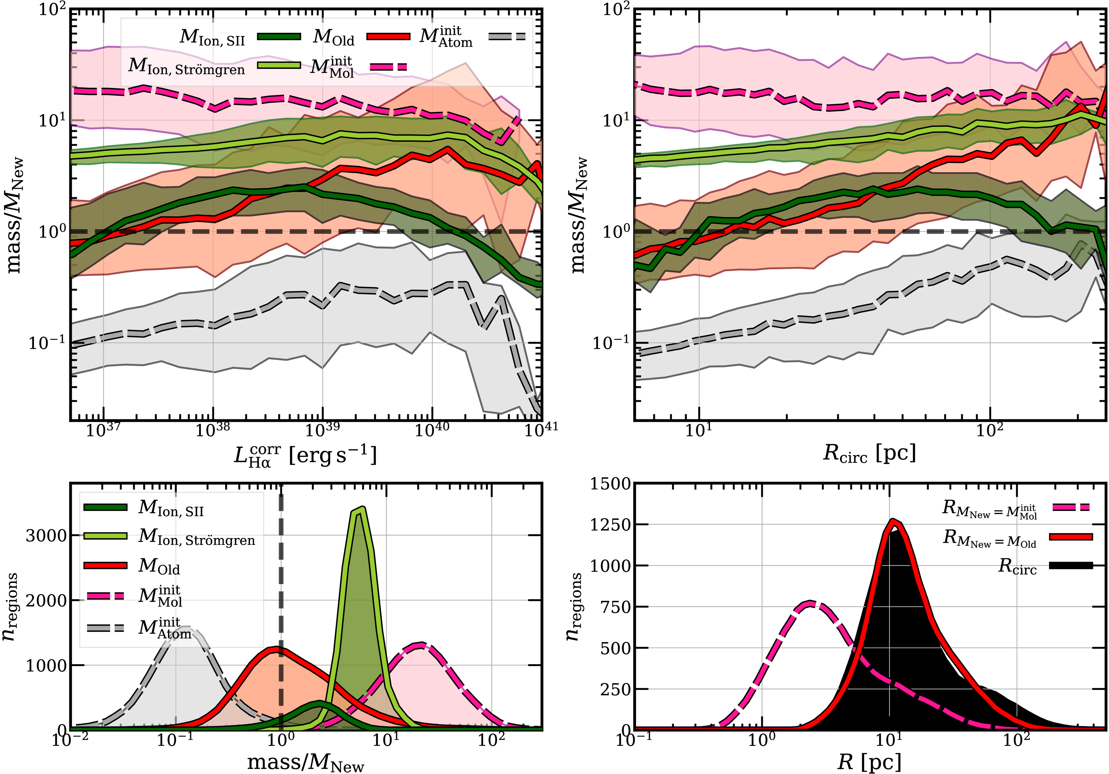
Figure 2. Variation in the different mass components relative to the young cluster mass MNew for the full sample of H II regions, binned in LHαcorr (top left) and Rcirc (top right) and summarized as histograms (bottom left). MIon, S II/MNew (dark green), ﹩{M}_{{\rm{Ion}}},{\rm{Str}}\ddot{{\rm{o}}}{\rm{mgren}}/{M}_{{\rm{New}}}﹩ (light green), MOld/MNew (red), ﹩{M}_{{\rm{Mol}}}^{{\rm{init}}}/{M}_{{\rm{New}}}﹩ (dashed pink), and ﹩{M}_{{\rm{Atom}}}^{{\rm{init}}}/{M}_{{\rm{New}}}﹩ (dashed gray) are included for comparison. The dashed line indicates where a mass component is equal to MNew. The bottom right panel includes the distribution of the measured Rcirc (black), the estimated radius at which ﹩{M}_{{\rm{New}}}={M}_{{\rm{Mol}}}^{{\rm{init}}}﹩ (dashed pink), and the radius where MNew = MOld (red).
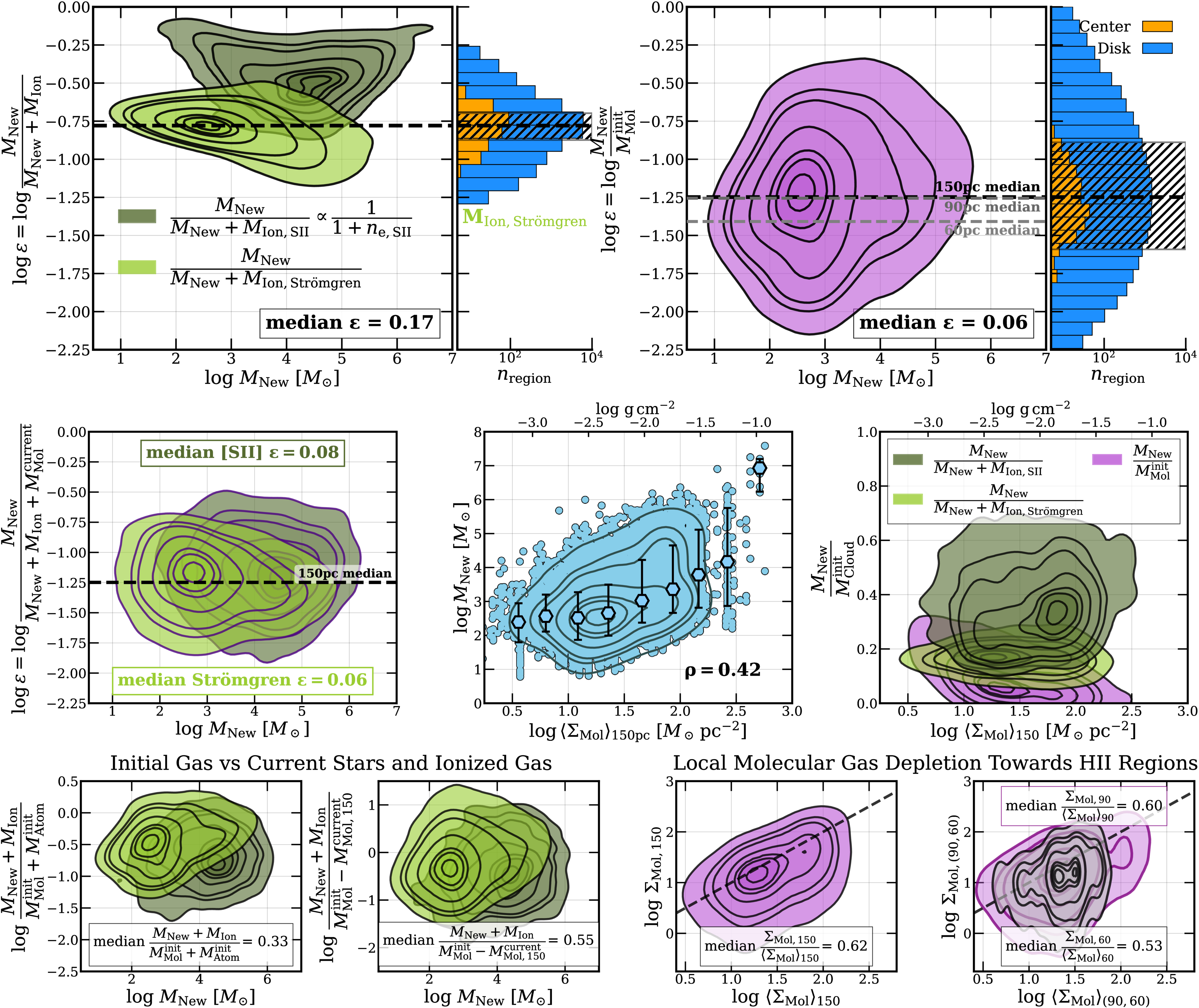
Figure 3. Top: summarizing H II region-scale SFEs. Data density contours for the 5th/16th/25th/50th/75th/84th/95th percentile SFE using MIon,S II (dark green), ﹩{M}_{{\rm{Ion}}},{\rm{Str}}\ddot{{\rm{o}}}{\rm{mgren}}﹩ (light green), and ﹩{M}_{{\rm{Mol}}}^{{\rm{init}}}﹩ (purple). The full histogram and medians as before (dashed line) for ﹩{M}_{{\rm{Ion}}},{\rm{Str}}\ddot{{\rm{o}}}{\rm{mgren}}﹩ and ﹩{M}_{{\rm{Mol}}}^{{\rm{init}}}﹩ are included. We also include the medians using ﹩{M}_{{\rm{Mol}}}^{{\rm{init}}}﹩ at 90–60 pc resolution. Middle: from left to right, the fraction of current gas and stars in young stars, the moderate correlation (Spearman ρ = 0.42) and large scatter between MNew and ﹩{\langle {{\rm{\Sigma }}}_{{\rm{Mol}}}\rangle }_{150\,{\rm{pc}}}﹩, and three estimates of MNew/MCloud vs. ﹩{\langle {{\rm{\Sigma }}}_{{\rm{Mol}}}\rangle }_{150\,{\rm{pc}}}﹩. Bottom: from left to right, the fraction of initial gas seen in stars and ionized gas, the fraction of depleted initial molecular gas in stars and ionized gas, the statistical local depletion in molecular gas toward H II regions at our fiducial 150 pc resolution, and finally, the depletion for smaller samples (where available) at 90 pc (purple) and 60 pc (gray) resolution, relative to the dashed black 1:1 line.
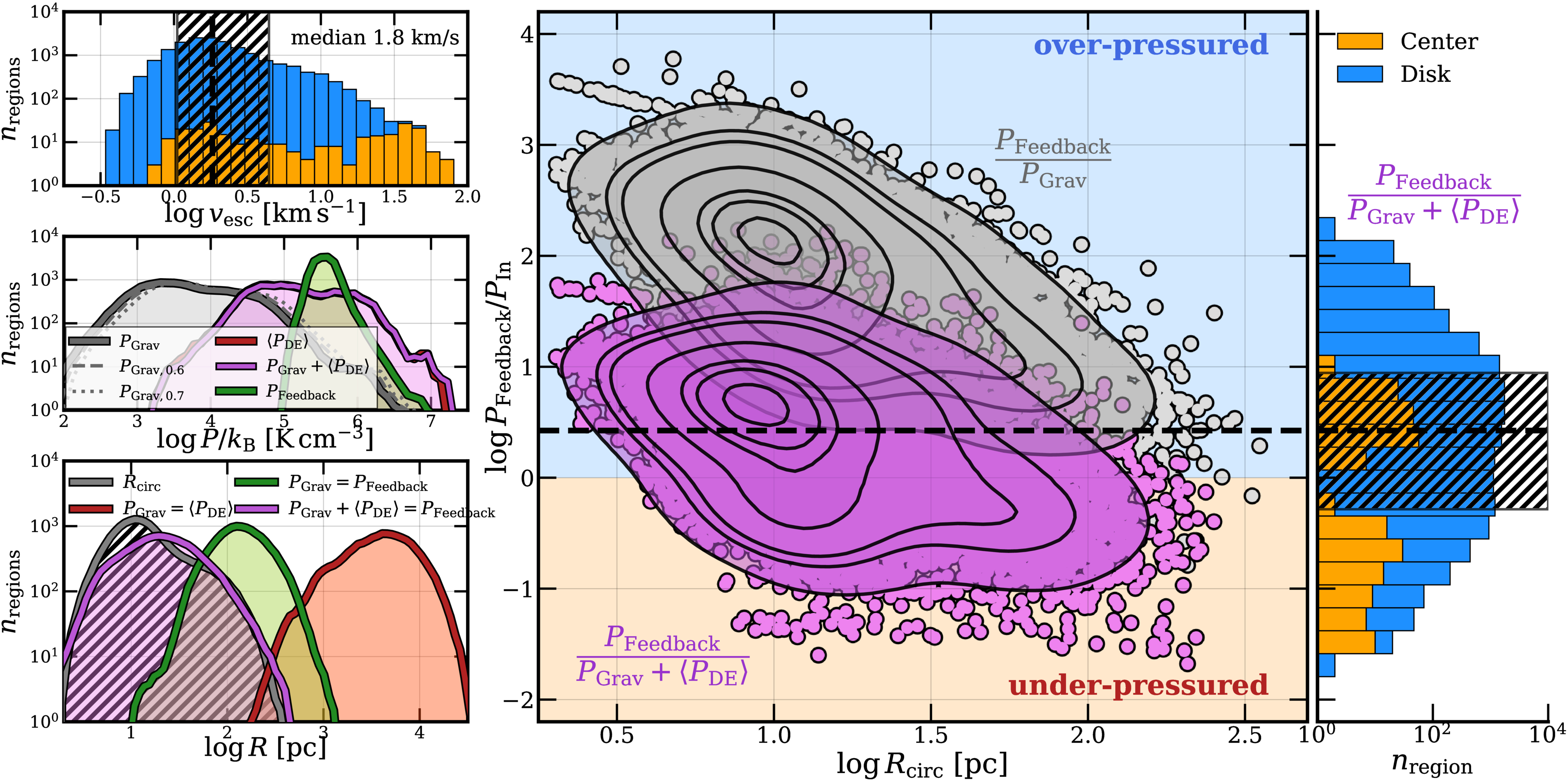
Figure 4. Top left: distribution of H II region escape velocities in galaxy centers and disks. Middle left: distribution of pressures due to H II region self-gravity for ﹩{M}_{{\rm{sh}}}=50 \% {M}_{{\rm{Mol}}}^{{\rm{init}}}﹩ (fiducial value; solid gray), ﹩60 \% {M}_{{\rm{Mol}}}^{{\rm{init}}}﹩ (dashed gray), and ﹩70 \% {M}_{{\rm{Mol}}}^{{\rm{init}}}﹩ (dotted–dashed gray); disk 〈PDE〉 (from J. Sun et al. 2023; maroon); fiducial PGrav + 〈PDE〉 (purple), and total PFeedback (green). Bottom left: distribution of H II region Rcirc (gray hatches) and the sizes at which we expect PGrav = 〈PDE〉 (maroon), PGrav = PFeedback (green), and PGrav + 〈PDE〉 = PFeedback (purple). Right: H II region overpressure (shaded blue) vs. underpressure (shaded orange) for PFeedback/PGrav (gray) and PFeedback/(PGrav + 〈PDE〉) (purple; the dashed line indicates the median, with a summary histogram to the right) with 5th/16th/25th/50th/75th/84th/95th percentile contours.