Linking stellar populations to HII regions across nearby galaxies. II. Infrared Reprocessed and UV Direct Radiation Pressure in HII Regions

Published in The Astrophysical Journal, Volume 982, Issue 2, id.140, 24 pp., 2025

Abstract

Radiation pressure is a key mechanism by which stellar feedback disrupts molecular clouds and drives H II region expansion. This includes direct radiation pressure exerted by UV photons on dust grains, pressure associated with photoionization, and infrared (IR) radiation pressure on grains due to dust-reprocessed IR photons. We present a new method that combines high-resolution mid-IR luminosities from JWST-MIRI, optical attenuation, and nebular line measurements from the Very Large Telecope Multi-Unit Spectroscopic Explorer (VLT-MUSE), and the Hubble Space Telescope (HST) Hα-based region sizes to estimate the strength of radiation pressure in ≍18,000 H II regions across 19 nearby star-forming galaxies. This is the most extensive and direct estimate of these terms beyond the Local Group to date. In the disks of galaxies, we find that the total reprocessed IR pressure is on average 5% of the direct UV radiation pressure. This fraction rises to 10% in galaxy centers. We expect reprocessed IR radiation pressure to dominate over UV radiation pressure in regions where . Radiation pressure due to H ionizations is lower than pressure on dust in our sample, but appears likely to dominate the radiation pressure budget in dwarf galaxies similar to the Small Magellanic Cloud. The contribution from all radiation pressure terms appears to be subdominant compared to thermal pressure from ionized gas, reinforcing the view that radiation pressure is most important in compact, heavily embedded, and young regions.

Figures

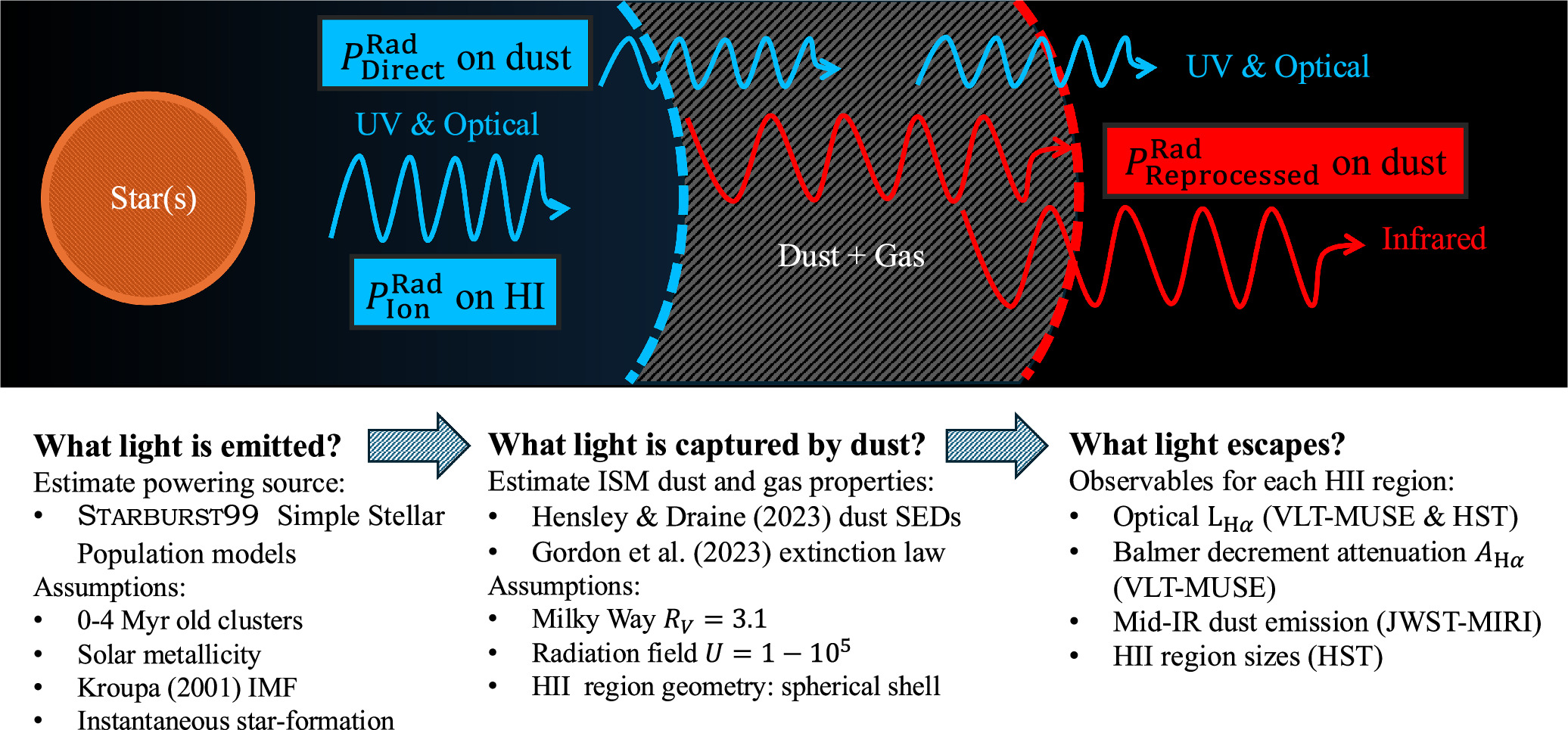
Figure 1. Radiation pressure in H II regions. UV and optical photons emitted from the central powering source interact with the surrounding dusty ISM. This results in ﹩{P}_{{\rm{Direct}}}^{{\rm{Rad}}}﹩ due to absorption and scattering off of dust grains and ﹩{P}_{{\rm{Ion}}}^{{\rm{Rad}}}﹩ due to H ionization. IR-reprocessed photons emitted by dust grains also interact with the dusty ISM. This results in an additional ﹩{P}_{{\rm{Reprocessed}}}^{{\rm{Rad}}}﹩ due to absorption of these IR photons by dust. With the assumptions indicated, Hα emission is used to estimate ﹩{P}_{{\rm{Ion}}}^{{\rm{Rad}}}﹩. Hα and the Balmer decrement extinction are used to estimate ﹩{P}_{{\rm{Direct}}}^{{\rm{Rad}}}﹩. Mid-IR dust emission and estimated mid-IR extinction are used to calculate ﹩{P}_{{\rm{Reprocessed}}}^{{\rm{Rad}}}﹩. See details in Section 3.
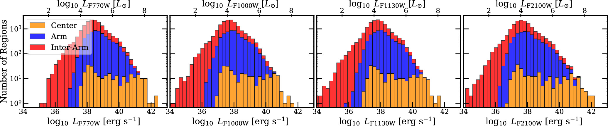
Figure 2. The distribution of filter-integrated luminosities LFX = ΔλFXLλ,FX for our sample of H II regions. We separate the regions by environment following M. Querejeta et al. (2021) and plot distributions for galactic centers (yellow), spiral arms and bars (blue), and inter-arm regions (red) separately. The panels show results for the four JWST-MIRI filters (FX) that we use—F770W, F1000W, F1130W, and F2100W.
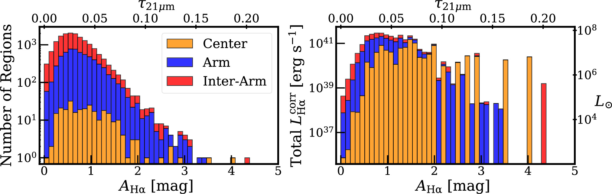
Figure 3. Left panel: the distribution of Hα attenuation, AHα, from VLT-MUSE (Section 2.1) in our sample of H II regions, colored by local environment as in Figure 2. The corresponding optical depth at 21 μm, τ21μm, converted from AHα using the G23 extinction law (Table 2), is included as an alternate x-axis. Right panel: corresponding ﹩{L}_{{\rm{H}}\alpha }^{{\rm{corr}}}﹩-weighted histograms, capturing how the Hα luminosity is distributed across regions of different attenuation.
Figure 4. Distribution of reprocessed radiation pressures ﹩{P}_{{\rm{Reprocessed}},{\rm{FX}}}^{{\rm{Rad}}}﹩ for each individual MIRI filter FX. We separate regions by local environment as in Figure 2. For the values of ﹩{P}_{{\rm{Reprocessed}}}^{{\rm{Rad}}}﹩ resulting from combining all filters and applying the SED-based correction described in Appendix B, see Figure 5.
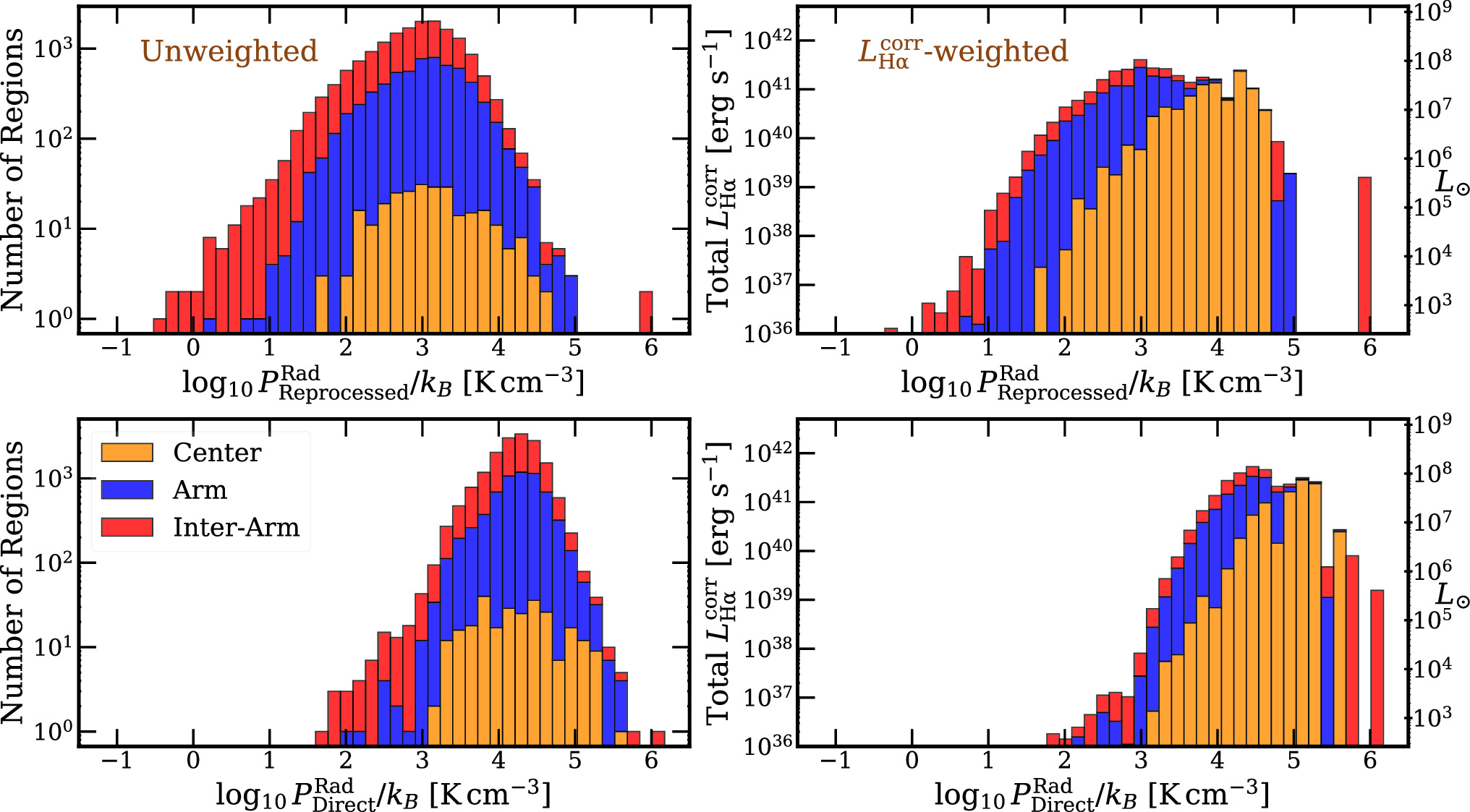
Figure 5. Distribution of total IR ﹩\mathrm{log}{P}_{\mathrm{Reprocessed}}^{\mathrm{Rad}}/{k}_{{\rm{B}}}﹩ (top) and UV-optical ﹩\mathrm{log}{P}_{\mathrm{Direct}}^{\mathrm{Rad}}/{k}_{{\rm{B}}}﹩ (bottom). Regions are again split by local environment—galactic centers (yellow), spiral arms and bars (blue), and inter-arm regions (red). The left panel treats each region equally, while the right panel weights regions by their ﹩{L}_{{\rm{H}}\alpha }^{{\rm{corr}}}﹩, similar to the right panel in Figure 3.
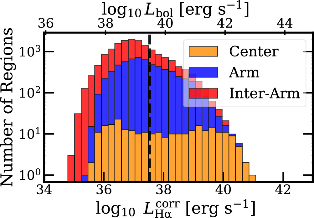
Figure 6. The distribution of attenuation-corrected ﹩{L}_{{\rm{H}}\alpha }^{{\rm{corr}}}﹩. The alternate x-axis shows the corresponding Lbol estimated by assuming the average ﹩{L}_{{\rm{bol}}}/{L}_{{\rm{H}}\alpha }^{{\rm{corr}}}﹩ ratio as described in Section 2.3 The vertical dashed line indicates the luminosity of a 1000 M⊙ SSP at the average age of our adopted model.
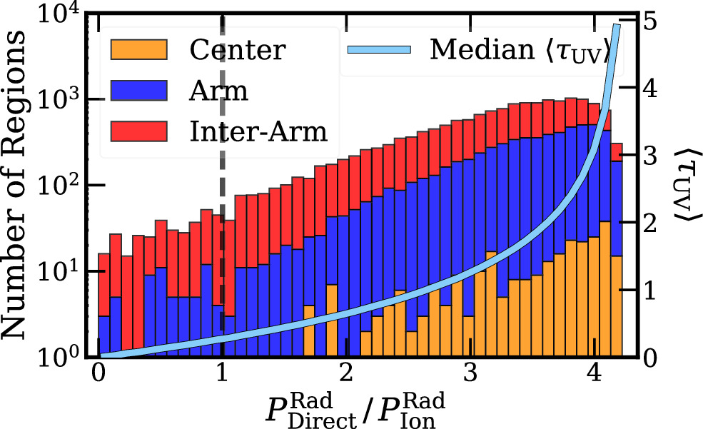
Figure 7. The distribution of ﹩{P}_{{\rm{Direct}}}^{{\rm{Rad}}}/{P}_{{\rm{Ion}}}^{{\rm{Rad}}}﹩ for our target regions split by local galactic environment. The light-blue line shows the median value of 〈τUV〉 (right y-axis) for the regions in each bin. The vertical dashed line indicates where ﹩{P}_{{\rm{Direct}}}^{{\rm{Rad}}}={P}_{{\rm{Ion}}}^{{\rm{Rad}}}﹩. This corresponds to 〈τUV〉 = 0.27.
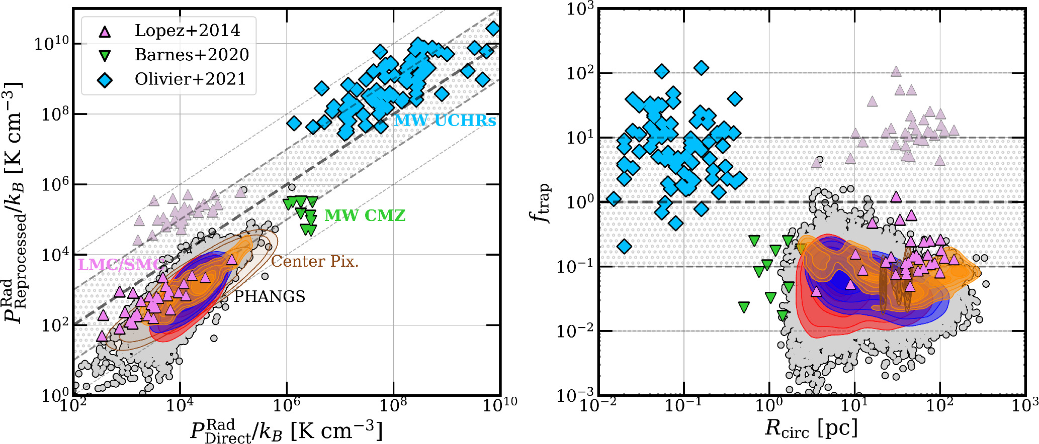
Figure 8. Left panel: ﹩{P}_{{\rm{Reprocessed}}}^{{\rm{Rad}}}﹩ and ﹩{P}_{{\rm{Direct}}}^{{\rm{Rad}}}﹩ for our ∼18,000 H II regions and literature measurements. Our individual regions are shown as gray points, and density contours represent the 16th–25th–50th–75th–84th percentile distributions colored by galactic environment—centers (yellow), spiral arms and bars (blue), and inter-arm regions (red). Brown contours show the data density for pixel-scale measurement in galactic centers (Section 2.3). Data from L. A. Lopez et al. (2014; LMC/SMC, purple triangles), G. M. Olivier et al. (2021; UCHRs, cyan diamonds), and A. T. Barnes et al. (2020; Milky Way CMZ, green triangles) is included for comparison. The original data from L. A. Lopez et al. (2014) appear as faint triangles, and bold triangles show their measurements after correcting for IR and UV optical depths (see Section 4). Right panel: similar to the left panel, now showing the variation in ﹩{f}_{{\rm{trap}}}={P}_{{\rm{Reprocessed}}}^{{\rm{Rad}}}/{P}_{{\rm{Direct}}}^{{\rm{Rad}}}﹩ as a function of region radius, Rcirc. The gray shaded region shows where the direct and reprocessed radiation pressure are within 1 dex of each other, around the dashed gray 1:1 line.
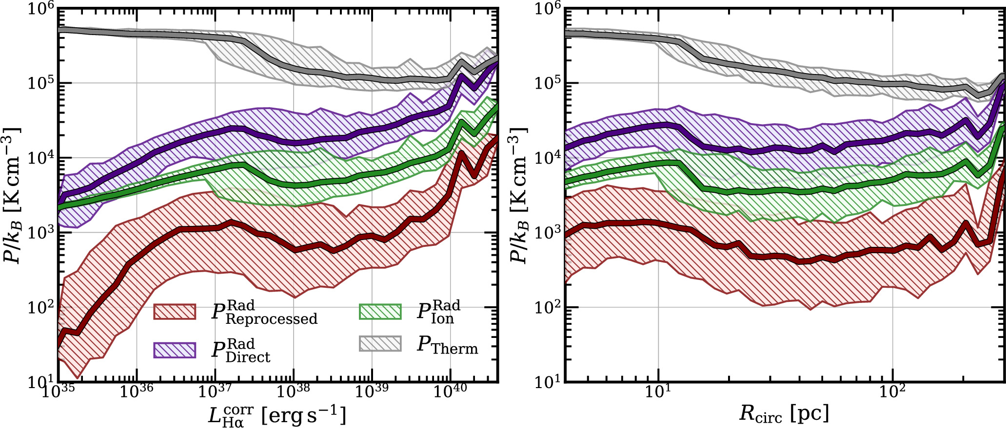
Figure 9. Here we compare ﹩{P}_{{\rm{Reprocessed}}}^{{\rm{Rad}}}﹩ (maroon), ﹩{P}_{{\rm{Direct}}}^{{\rm{Rad}}}﹩ (navy), ﹩{P}_{{\rm{Ion}}}^{{\rm{Rad}}}﹩ (green), and the Strömgren PTherm (gray) for the full sample of H II regions. The hatched regions show the 16th–84th percentiles, and the solid lines show the median of each radiation pressure term. Variation of the pressures with ﹩{L}_{{\rm{H}}\alpha }^{{\rm{corr}}}﹩ (left panel) and Rcirc (right panel) for each region is included for comparison.
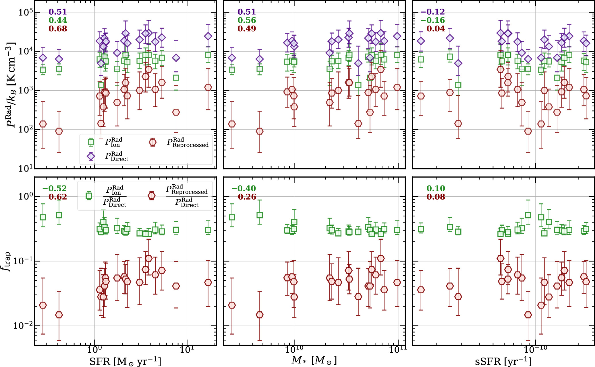
Figure 10. Here we compare the median﹩{P}_{{\rm{Reprocessed}}}^{{\rm{Rad}}}﹩ (maroon hexagons), ﹩{P}_{{\rm{Direct}}}^{{\rm{Rad}}}﹩ (blue diamonds), and ﹩{P}_{{\rm{Ion}}}^{{\rm{Rad}}}﹩ (green squares; top row), and ﹩{f}_{{\rm{trap}}}={P}_{{\rm{Reprocessed}}}^{{\rm{Rad}}}/{P}_{{\rm{Direct}}}^{{\rm{Rad}}}﹩ (maroon hexagons) and ﹩{P}_{{\rm{Ion}}}^{{\rm{Rad}}}/{P}_{{\rm{Direct}}}^{{\rm{Rad}}}﹩ (green squares; bottom row) with the average star formation rate (SFR), total stellar mass (M*), and specific star formation rate (sSFR) for all 19 galaxies. Each marker shows the median for each galaxy, and the error bars denote the 16th–84th percentile range in values. The Spearman rank coefficient ρ for the correlation between each median and galaxy property is noted in the top left of each panel.
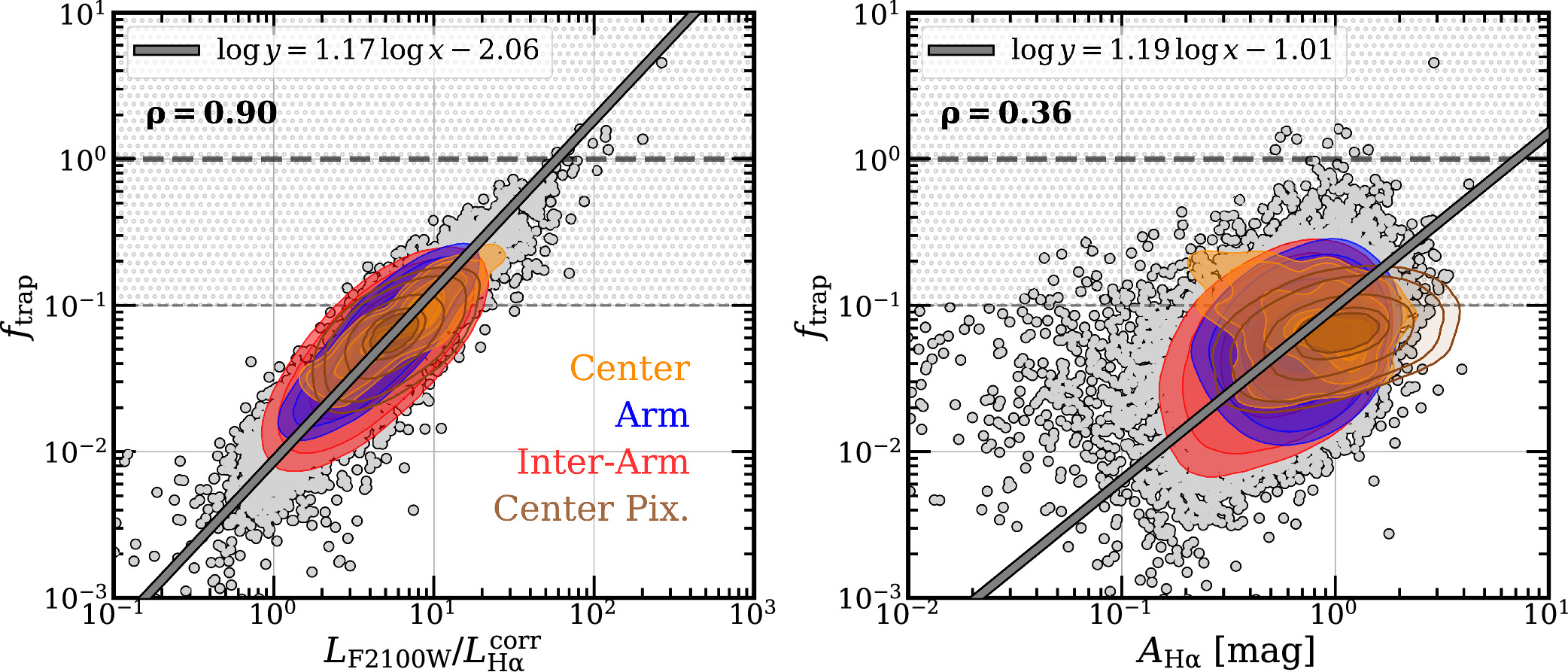
Figure 11. Variation in ftrap as a function of ﹩{L}_{{\rm{F2100W}}}/{L}_{{\rm{H}}\alpha }^{{\rm{corr}}}﹩, which roughly captures the shape of the SED (left panel) and attenuation AHα, with corresponding ﹩\mathrm{log}\unicode{8210}\mathrm{log}﹩ bisector fits (solid black line). Individual regions are shown as gray background points, and density contours represent the 16th–25th–50th–75th–84th percentile distributions colored by local environment—galaxy centers (yellow), spiral arms (blue), inter-arm regions (red). Brown contours show the distribution of ﹩0\mathop{.}\limits^{^{\prime\prime} }9﹩ pixel-scale MUSE estimates in galaxy centers. ftrap shows a tight empirical correlation with ﹩{L}_{{\rm{F2100W}}}/{L}_{{\rm{H}}\alpha }^{{\rm{corr}}}﹩, and shows much more scatter with attenuation. The gray shaded area shows the region where the direct and reprocessed radiation pressure terms are within 1 dex of each other, around the dashed gray line where ftrap = 1. The Spearman rank coefficient ρ for the full sample of regions is included.
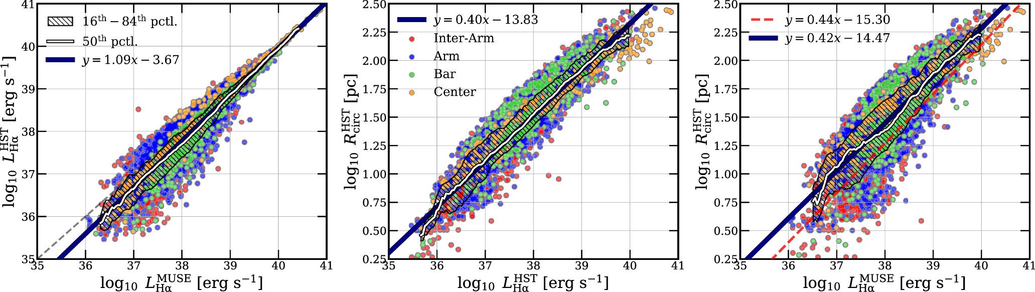
Figure 12. Correlations between (left panel) Hα luminosity in erg s−1, as measured by MUSE and HST, (center panel) HST size and HST Hα luminosity from A. Barnes et al. (2025, in preparation), and (right panel) the closure relation between MUSE luminosities and HST sizes. All panels show the 7082 H II regions with joint HST and MUSE coverage. Individual regions are colored by their local environment—galactic centers (yellow), bars (green), spiral arms (blue), and inter-arm regions or the disk (red). The solid white line traces the 50th percentile in y for each bin along the x-axis, and the 16th–84th percentile scatter in each bin is indicated with black hatches. Finally, the best-fit log–log correlation is shown in dark blue, which follows the 50th percentile relation very closely. The gray dashed line indicates the 1:1 line in the left panel, and the red dashed line in the right panel shows the convolution of Equations (A1) and (A3).
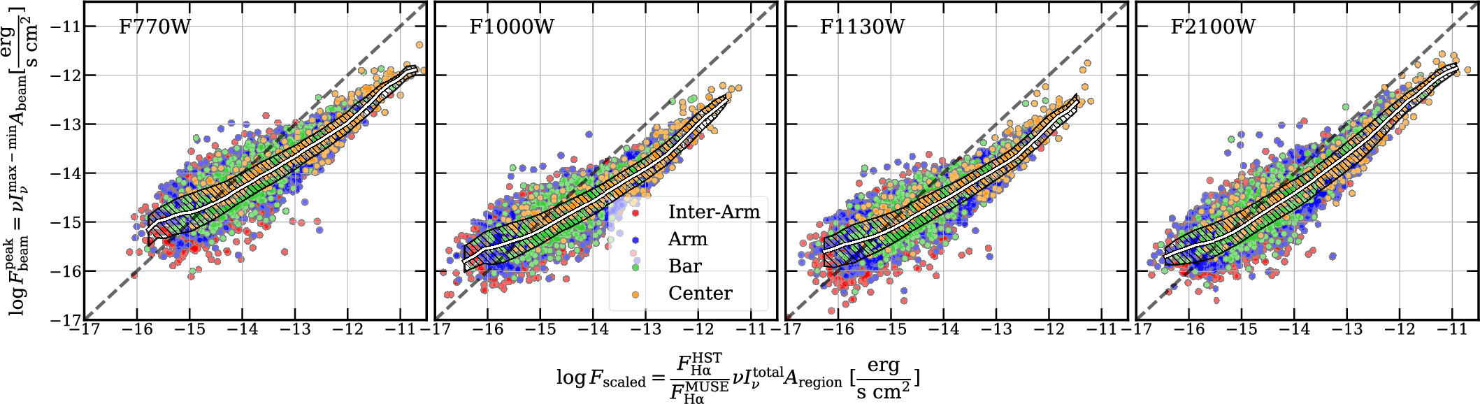
Figure 13. Comparing two methods for re-scaling MIRI fluxes from MUSE regions to HST for the  ∼7000 H II regions with full HST, MUSE, and JWST-MIRI coverage, colored by local environment. The x-axis scales MIRI fluxes directly by the same proportion that MUSE Hα fluxes are scaled relative to HST Hα fluxes. The y-axis calculates the total flux associated with a point source with peak intensity corresponding to the brightest pixel in each region, with a local background subtraction in each region, at ﹩0\mathop{.}\limits^{^{\prime\prime} }9﹩ resolution.
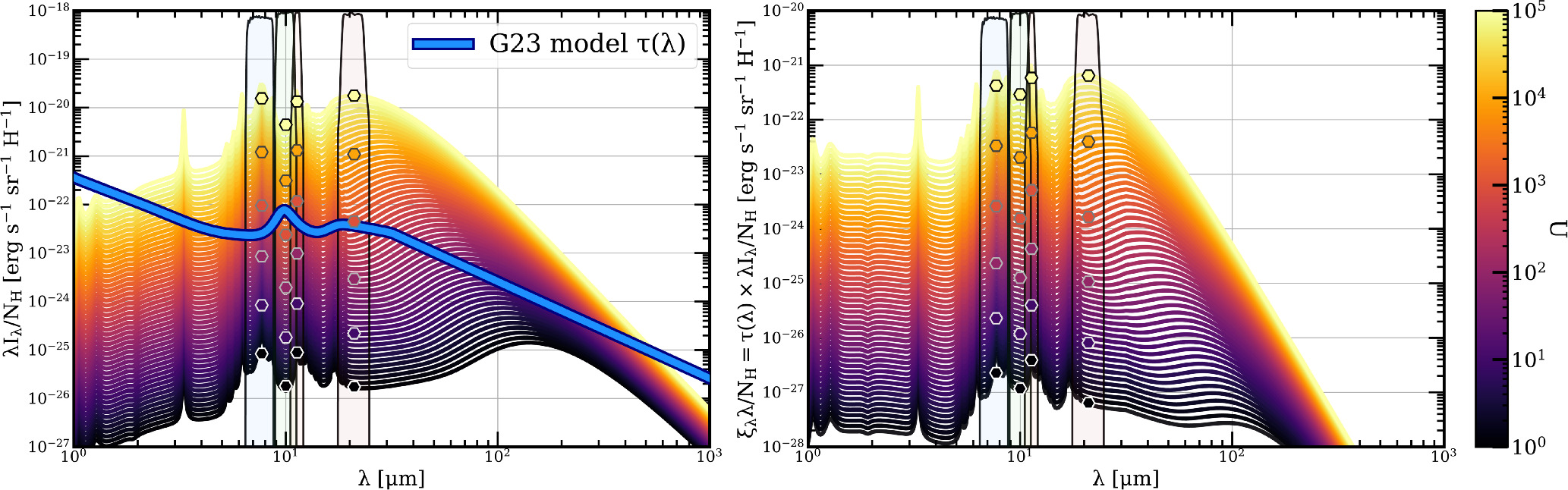
Figure 14. Standard HD23 dust models at different radiation fields U. The G23 extinction curve (arbitrary normalization, for visualization only), and the MIRI filter throughputs (arbitrary normalization) at F770W, F1000W, F1130W, and F2100W are included. The left panel shows the variation in intensity λIλ with wavelength and U, showing how the SED of dust emission changes with radiation field. The right panel shows how the shape of the optical depth-weighted intensity, λξλ = τ(λ)λIλ, which is a proxy for pressure contribution, varies with U. Hexagonal points represent the shape of the measured SED by showing the model SED convolved with each of the four MIRI bandpasses, at U = 1, 10, 102, 103, 104,  and 105.
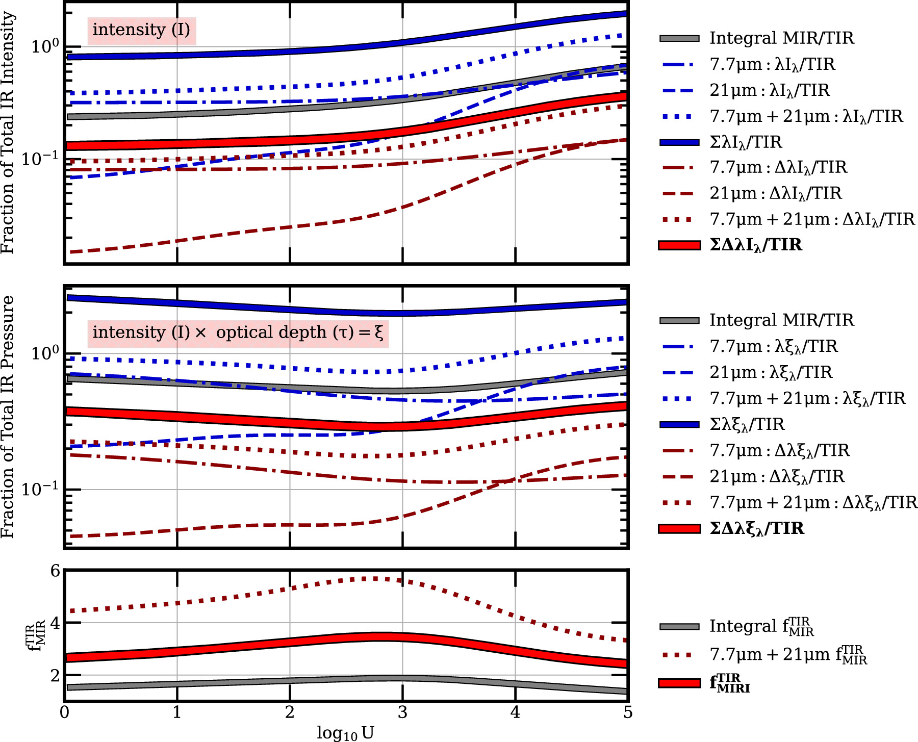
Figure 15. Top panel: the fraction of total IR intensity (or flux) (TIR﹩={\int }_{1\,\mu {\rm{m}}}^{1000\,\mu {\rm{m}}}{I}_{\lambda }d\lambda ﹩) captured by different approximations and linear combinations of MIRI filters at a range of U. First, we present the fraction of TIR flux captured by the λIλ approximation in the 7.7 μm filter (blue dotted–dashed), 21 μm filter (blue dashed), 7.7 μm + 21 μm filters (blue dotted), and all four MIRI filters (solid blue). Next, using the filter width Δλ for each MIRI filter, we present the fraction captured by ΔλIλ in the 7.7 μm filter (red dotted–dashed), 21 μm (red dashed), 7.7 μm + 21 μm filters (red dotted), and adding all four MIRI filters (solid red). Finally, we present the fraction of flux captured in the mid-IR by an integral over the model dust SED as ﹩{\int }_{1\mu {\rm{m}}}^{25\mu {\rm{m}}}{I}_{\lambda }d\lambda /{\int }_{1\mu {\rm{m}}}^{1000\mu {\rm{m}}}{I}_{\lambda }d\lambda ﹩ (solid gray). Middle panel: similar to the top panel, now for opacity-weighted intensity (proxy for pressure) ξλ instead of intensity Iλ. Bottom panel: inverting the fractions in the middle panel provides the mid-IR to TIR correction factor ﹩{f}_{\xi }^{{\rm{TIR}}}﹩ at a given U. The correction factor from integrating the model SED (solid gray), adding up all four MIRI filters (solid red), and 7.7 μm + 21 μm filters (red dotted) is included for comparison. The MIRI-estimated ﹩{f}_{\xi }^{{\rm{TIR}}}﹩ using all four filters (solid red) is used for all ﹩{P}_{{\rm{Reprocessed}}}^{{\rm{Rad}}}﹩ calculations.
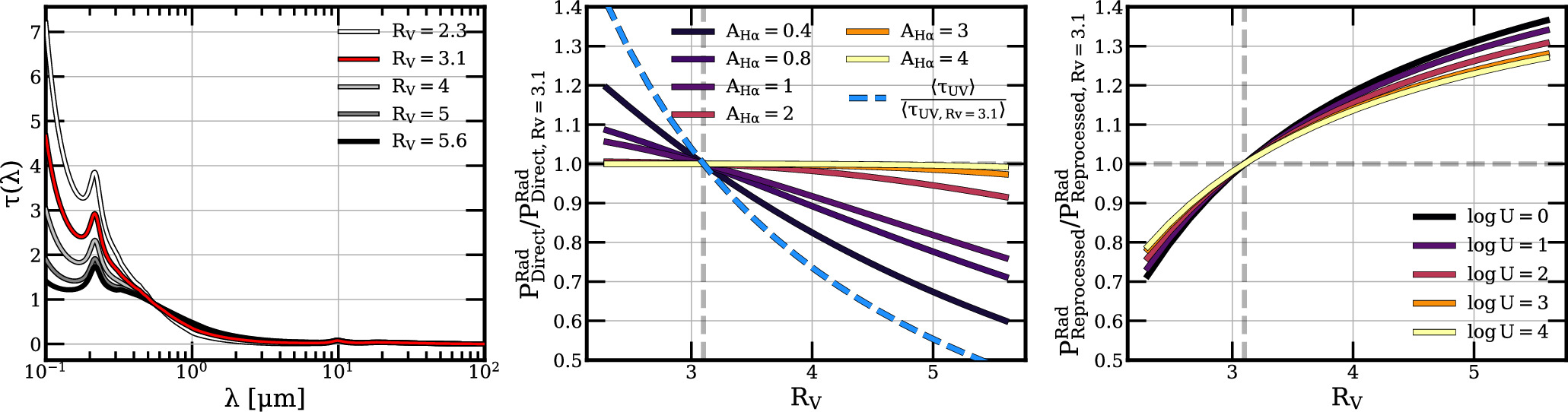
Figure 16. The impact of variation in RV. Left panel: variation of the K. D. Gordon et al. (2023) extinction curves as a function of RV. Additionally, the center panel shows the scaling of ﹩{P}_{{\rm{Direct}}}^{{\rm{Rad}}}﹩ while the right panel shows ﹩{P}_{{\rm{Reprocessed}}}^{{\rm{Rad}}}﹩ as a function of RV for values between 2.3 and 5.6, normalized to a our fiducial RV of 3.1. The variation in ﹩{P}_{{\rm{Direct}}}^{{\rm{Rad}}}﹩ relative to RV = 3.1 depends on the attenuation, and we show a range of AHα between 0.4 and 4. The relative variation in ﹩{P}_{{\rm{Reprocessed}}}^{{\rm{Rad}}}﹩ depends to a smaller degree on the radiation field, shown for a range of log U between 0 and 4.